
Tips & Shortcuts in Excel (Part 4)
Our final Tech Tip for this month will explain how to make your data look nice, organized, and visually appealing. Whether you are adding graphs, making the data itself look nice and neat, or giving the worksheet the last finishing touches – you can find it all in the article below!
Visualize your data with the Quick Analysis tool
You can instantly create different types of charts, including line and column charts, or add miniature graphs (called Sparklines). You can also apply a table style, create PivotTables, quickly insert totals, and apply conditional formatting.
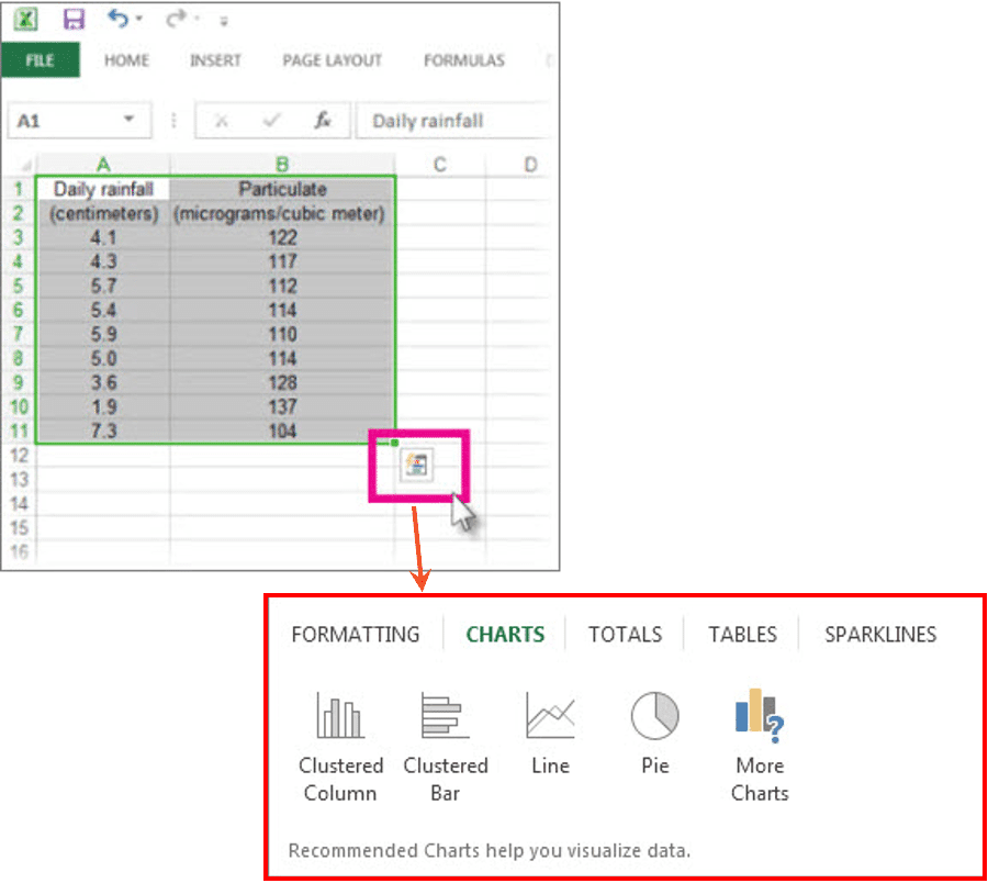
- Select the cells that contain the data you want to analyze.
- Right-click the selected cells and click the Quick Analysis button image button that appears to the bottom right of your selected data (or press CRTL + Q).
- In the Quick Analysis gallery, select a tab you want. For example, select “Charts” to see your data displayed in a chart.
- Pick an option, or hover over each one to see a preview.
You might notice that the options you can choose from aren’t always the same. That is because the options change based on the type of data you have selected in your workbook.
If you’re not sure which analysis option to pick, here’s a quick overview:
- Formatting – lets you highlight parts of your data by adding things like data bars and colors. This lets you quickly see high and low values, among other things.
- Charts – Excel recommends different charts, based on the type of data you have selected. If you don’t see the chart you want, click More Charts.
- Totals – lets you calculate the numbers in columns and rows. For example, Running Total inserts a total that grows as you add items to your data. Click the little black arrows on the right and left to see additional options.
- Tables – make it easy to filter and sort your data. If you don’t see the table style you want, click More.
- Sparklines – are tiny graphs that you can show alongside your data. They provide a quick way to see trends.
Combine cell content
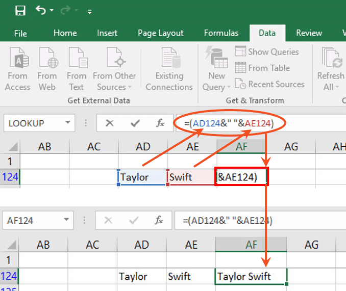
- Click the cell where you want the text string to appear.
- To start the string, type “=(“.
- To combine the contents of two cells, click the first cell that contains the text that you want to combine, type &” “& (a space enclosed in quotation marks), and then click the next cell that contains the text that you want to combine.
- To combine the contents of more than two cells, continue selecting cells, making sure to type &” “& after you select each cell.
- If you don’t want to add a space between combined text, type & instead of &” “&.
- To insert a comma, type &”, “& (a comma followed by a space, both enclosed in quotation marks).
- To complete the formula, type ) and, finally, to see the results of the formula, press ENTER.
Quickly add a Header & Footer
Excel has many built-in headers and footers that you can use. For worksheets, you can work with headers and footers in the Page Layout view, or you can just choose from the many built-in elements found in the ribbon.

Add a built-in header or footer to a worksheet in Page Layout view
- Click the worksheet to which you want to add a predefined header or footer.
- On the Insert tab, in the Text group, click Header & Footer (Box 1).
- Click the left, center, or right header or footer text box at the top or the bottom of the worksheet page. Clicking any text box selects the header or footer and displays the Header and Footer Tools, adding the Design tab (Box 2).
- On the Design tab, in the Header & Footer group (Box 3), chose Header or Footer, and then click the predefined header or footer that you want.
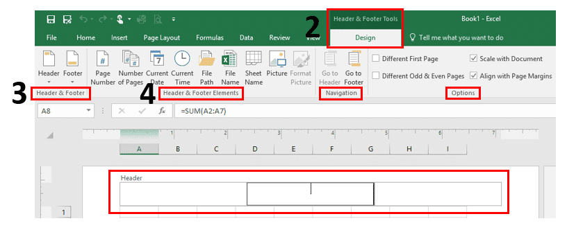
Inserting built-in header and footer elements for a worksheet:
- Repeat steps 1 through 3 mentioned above.
- On the Design tab, in the Header & Footer Elements group (Box 4), click the elements that you want.
Closing headers and footers:
To close the header and footer, you must switch from Page Layout view to Normal view.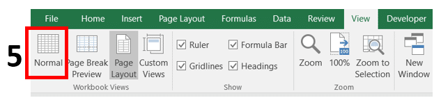
- On the View tab, in the Workbook Views group, click Normal (Box 5).
- You can also click Normal Button image on the status bar.

Our Free Microsoft Office 365 Hands-On Workshops are back!
Join us for our Free Microsoft Office 365 Hands-On Workshops at our Main Office (441 E Hector Street, 3rd Floor, Conshohocken, PA 19428), where we offer you a hands-on environment in which you can test-drive best-in-class Microsoft technologies, including Windows 10, Office 365, Skype for Business, SharePoint, OneDrive, and more – all while working on the newest and coolest Windows devices.
Click here to learn more and sign up.