
Tips & Shortcuts in Excel (Part 3)
It’s all about minimizing efforts and maximizing output these days! Today’s Tech Tip explains how to make certain “auto” features work for you when crunching numbers and analyzing data.
AutoSum and Quick Sum with the Status Bar
To quickly get the Sum of a range of cells, all you need to do is select the range, and then click AutoSum—even quicker, select the range of cells and look in the lower right-hand side of the Excel window, the so-called Status Bar (more detail to follow).
AutoSum from the Ribbon:
- Select the range of cells you would like to get the sum of by highlighting those cells.
- Select an empty cell to the right or below the numbers you want to add, then click AutoSum on the Home tab (Box 1).

(Note: Click the drop-down link to the right of the AutoSum button for more options besides Sum.)
Quick Sum with the Status Bar…
- If you want to quickly get the Sum of a range of cells, all you need to do is select the range of cells (by highlighting them) and look in the lower right-hand side of the Excel window (Box 1).
- If you then right-click on the Status Bar, a feature dialog box will pop out displaying all of your options.
(Note: It also displays values for your selected range if you have those attributes checked.)
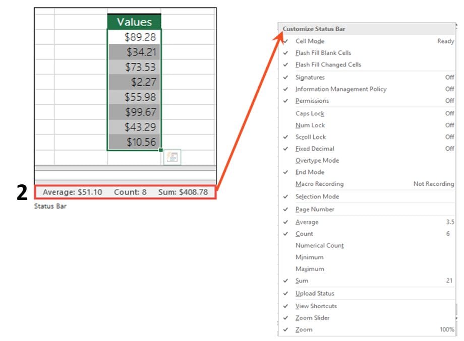
(Note: This is the Status Bar, and it displays information regarding whatever you have selected, whether it’s a single cell or multiple cells.)
Use Auto Fill
Instead of entering data manually into a worksheet, you can use the Auto Fill feature to fill cells with data that follows a pattern or that is based on data in other cells.
Filling data into adjacent cells by using the Fill Handle: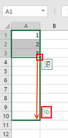
To quickly fill in several types of data series, you can select cells and drag the fill handle. In this example, the Fill Handle is located at the lower-right-hand corner of cell #3.
- To use the Fill Handle, you select the cells that you want to use as a basis for filling additional cells
- Then, drag the fill handle across or down the cells that you want to fill (down to cell #10, in this example).
- After you drag the fill handle, the Auto Fill Options button is displayed (box 1).
- To change how you want to fill the selection, click the Auto Fill Options Button, and then click your preferred option.
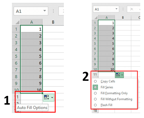
(Note: If you don’t want to display the Auto Fill Options button every time that you drag the fill handle, you can turn it off. Likewise, if the Auto Fill Options button does not appear when you drag the fill handle, you have the option to turn it on.)
(Note: If you drag the fill handle up or to the left of a selection and stop in the selected cells without going past the first column (to the grey numbered section) or the top row in the selection (to the grey lettered section), Excel deletes the data within the selection. You must drag the fill handle out of the selected area before releasing the mouse button.)
Use Flash Fill
When you need to enter a lot of repetitive information in Excel, such as dates, the AutoFill feature can help; however, when you need to quickly split a single column of data into multiple columns, Flash Fill can do the work for you. Flash Fill recognizes patterns in your data, and completes the data accordingly.
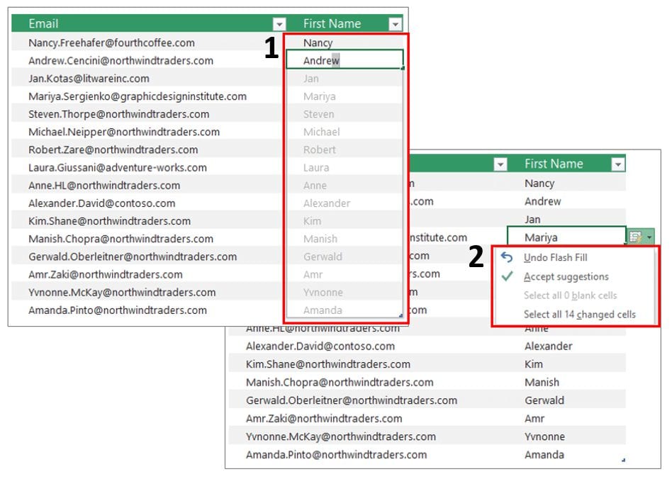
Example: You have a list of names that is not formatted the way you need it, or that you want to separate (like the first name from an email address):
- Start by typing the first name the way you want it (into the First Name column).
- Then, start typing the next name into the next cell down, and Excel provides a preview of the names formatted the way you want (Box 1).
- Press Enter and Flash Fill will fill-in the names for you.
- Once the data is filled-in, Flash Fill provides a drop-down box with various options you can apply to your data (Box 2).
(Note: Flash Fill works best on consistent data, and doesn’t work on text that is mistyped, e.g. inconsistent capitalization, like “Nancy” vs. “nancy”.)
Transpose your data
When you have an Excel worksheet with data in columns that you want to rearrange into rows instead—or vice versa—Excel’s Transpose feature can help you do that.
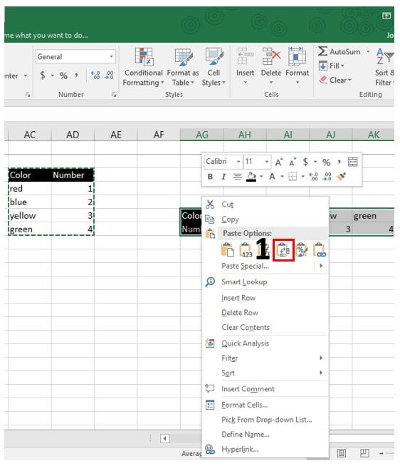
- Select the range of data you want to rearrange, including any row or column labels, and copy it (either right-click > copy, or Ctrl+C).
- Next, pick a spot in the worksheet that has enough room to paste your data.
- Then, right-click the first cell where you want to paste the data, and select the symbol for Transpose within the “Paste Options”.
- The data you copied will overwrite any data that’s already there.

Our Free Microsoft Office 365 Hands-On Workshops are back!
Join us for our Free Microsoft Office 365 Hands-On Workshops at our Main Office (441 E Hector Street, 3rd Floor, Conshohocken, PA 19428), where we offer you a hands-on environment in which you can test-drive best-in-class Microsoft technologies, including Windows 10, Office 365, Skype for Business, SharePoint, OneDrive, and more – all while working on the newest and coolest Windows devices.
Click here to learn more and sign up.